STAC + stackstac + xarray

stackstac is a python package for making it dead simple to process data from a STAC using xarray.

When you use stackstac, you do not need to write any code to handle merging operations for many raster files. The data come out the other side in a neatly packaged xarray object with x, y, time, and band dimensions! This is very convenient when you are interested in an arbitrary area that may require combining data from many STAC items. The stackstac documentation is very good, but I have put this demo together to highlight a few things that I really like about the STAC + stackstac + xarray workflow.

Define search parameters

I am interested in getting a mosaic of daily observations from Sentinel 2 for September 2022.

import pyproj
import pystac_client
import stackstac
import xarray as xr
from shapely.geometry import box
from shapely.ops import transform

# STAC connection information for Sentinel 2 COGs
STAC_URL = "https://earth-search.aws.element84.com/v0"
STAC_COLLECTION = "sentinel-s2-l2a-cogs"

# spatial projection information
CRS_STRING = "epsg:5070"
EPSG = pyproj.CRS.from_string(CRS_STRING).to_epsg()

# area of interest along the North Shore of Lake Superior
AOI = box(373926, 2744693, 406338, 2765304)

# a few more parameters
RESOLUTION = 100  # meters
BANDS = ["B04", "B03", "B02"]
START_DATE = "2022-09-01"
END_DATE = "2022-09-30"

Query the STAC for matching items

To query the STAC, we need to provide a bounding box in epsg:4326 coordinates:

# STAC items store bounding box info in epsg:4326
transformer_4326 = pyproj.Transformer.from_crs(
    crs_from=CRS_STRING,
    crs_to="epsg:4326",
    always_xy=True,
)

bbox_4326 = transform(transformer_4326.transform, AOI).bounds

This will return all of the STAC items that intersect the provided bounding box and time window:

catalog = pystac_client.Client.open(STAC_URL)

stac_items = catalog.search(
    collections=[STAC_COLLECTION],
    bbox=bbox_4326,
    datetime=[START_DATE, END_DATE],
).get_all_items()

The query yields many STAC items, each of which describes multiple COGs (one per band). Using other tools, we would need to write a bunch of code to make sure we combine the data correctly but with stackstac we can forget about that and just get on with our analysis!

len(stac_items)

20

Stack it

Lazily load the raster data into an xarray.DataArray using stackstack.stack. This function uses the STAC item metadata to construct a multidimensional array with human-readable coordinates that can be manipulated with the magnificently powerful suite of xarray functions and methods!

sentinel_stack = stackstac.stack(
    items=stac_items,
    assets=BANDS,
    epsg=EPSG,
    resolution=RESOLUTION,
    bounds=AOI.bounds,
    xy_coords="center",
)
sentinel_stack

/opt/hostedtoolcache/Python/3.11.4/x64/lib/python3.11/site-packages/stackstac/prepare.py:363: UserWarning: The argument 'infer_datetime_format' is deprecated and will be removed in a future version. A strict version of it is now the default, see https://pandas.pydata.org/pdeps/0004-consistent-to-datetime-parsing.html. You can safely remove this argument.
  times = pd.to_datetime(

<xarray.DataArray 'stackstac-d46fb9a7b2a8799953cea62902a886ed' (time: 20,
                                                                band: 3,
                                                                y: 208, x: 325)>
dask.array<fetch_raster_window, shape=(20, 3, 208, 325), dtype=float64, chunksize=(1, 1, 208, 325), chunktype=numpy.ndarray>
Coordinates: (12/29)
  * time                          (time) datetime64[ns] 2022-09-03T17:10:24 ....
    id                            (time) <U24 'S2B_15UXP_20220903_0_L2A' ... ...
  * band                          (band) <U3 'B04' 'B03' 'B02'
  * x                             (x) float64 3.74e+05 3.74e+05 ... 4.064e+05
  * y                             (y) float64 2.765e+06 2.765e+06 ... 2.745e+06
    constellation                 <U10 'sentinel-2'
    ...                            ...
    title                         (band) <U14 'Band 4 (red)' ... 'Band 2 (blue)'
    proj:shape                    object {10980}
    common_name                   (band) <U5 'red' 'green' 'blue'
    center_wavelength             (band) float64 0.6645 0.56 0.4966
    full_width_half_max           (band) float64 0.038 0.045 0.098
    epsg                          int64 5070
Attributes:
    spec:        RasterSpec(epsg=5070, bounds=(373900, 2744600, 406400, 27654...
    crs:         epsg:5070
    transform:   | 100.00, 0.00, 373900.00|\n| 0.00,-100.00, 2765400.00|\n| 0...
    resolution:  100

xarray.DataArray

'stackstac-d46fb9a7b2a8799953cea62902a886ed'

• time: 20
• band: 3
• y: 208
• x: 325

• dask.array<chunksize=(1, 1, 208, 325), meta=np.ndarray>

  Array Chunk Bytes 30.94 MiB 528.12 kiB Shape (20, 3, 208, 325) (1, 1, 208, 325) Dask graph 60 chunks in 3 graph layers Data type float64 numpy.ndarray

• Coordinates: (29)
  • time
    (time)
    datetime64[ns]
    2022-09-03T17:10:24 ... 2022-09-...

    array(['2022-09-03T17:10:24.000000000', '2022-09-03T17:10:34.000000000',
           '2022-09-06T17:20:16.000000000', '2022-09-06T17:20:29.000000000',
           '2022-09-08T17:10:30.000000000', '2022-09-08T17:10:44.000000000',
           '2022-09-13T17:10:20.000000000', '2022-09-13T17:10:35.000000000',
           '2022-09-16T17:20:17.000000000', '2022-09-16T17:20:30.000000000',
           '2022-09-18T17:10:27.000000000', '2022-09-18T17:10:41.000000000',
           '2022-09-21T17:20:23.000000000', '2022-09-21T17:20:36.000000000',
           '2022-09-23T17:10:19.000000000', '2022-09-23T17:10:34.000000000',
           '2022-09-26T17:20:22.000000000', '2022-09-26T17:20:29.000000000',
           '2022-09-28T17:10:26.000000000', '2022-09-28T17:10:40.000000000'],
          dtype='datetime64[ns]')

  • id
    (time)
    <U24
    'S2B_15UXP_20220903_0_L2A' ... '...

    array(['S2B_15UXP_20220903_0_L2A', 'S2B_15TXN_20220903_0_L2A',
           'S2B_15UXP_20220906_0_L2A', 'S2B_15TXN_20220906_1_L2A',
           'S2A_15UXP_20220908_0_L2A', 'S2A_15TXN_20220908_0_L2A',
           'S2B_15UXP_20220913_0_L2A', 'S2B_15TXN_20220913_0_L2A',
           'S2B_15UXP_20220916_0_L2A', 'S2B_15TXN_20220916_0_L2A',
           'S2A_15UXP_20220918_0_L2A', 'S2A_15TXN_20220918_0_L2A',
           'S2A_15UXP_20220921_1_L2A', 'S2A_15TXN_20220921_0_L2A',
           'S2B_15UXP_20220923_0_L2A', 'S2B_15TXN_20220923_0_L2A',
           'S2B_15UXP_20220926_1_L2A', 'S2B_15TXN_20220926_1_L2A',
           'S2A_15UXP_20220928_0_L2A', 'S2A_15TXN_20220928_0_L2A'],
          dtype='<U24')

  • band
    (band)
    <U3
    'B04' 'B03' 'B02'

    array(['B04', 'B03', 'B02'], dtype='<U3')

  • x
    (x)
    float64
    3.74e+05 3.74e+05 ... 4.064e+05

    array([373950., 374050., 374150., ..., 406150., 406250., 406350.])

  • y
    (y)
    float64
    2.765e+06 2.765e+06 ... 2.745e+06

    array([2765350., 2765250., 2765150., ..., 2744850., 2744750., 2744650.])

  • constellation
    ()
    <U10
    'sentinel-2'

    array('sentinel-2', dtype='<U10')

  • sentinel:product_id
    (time)
    <U60
    'S2B_MSIL2A_20220903T165849_N040...

    array(['S2B_MSIL2A_20220903T165849_N0400_R069_T15UXP_20220903T214148',
           'S2B_MSIL2A_20220903T165849_N0400_R069_T15TXN_20220903T214148',
           'S2B_MSIL2A_20220906T170849_N0400_R112_T15UXP_20220906T210522',
           'S2B_MSIL2A_20220906T170849_N0400_R112_T15TXN_20220906T210522',
           'S2A_MSIL2A_20220908T165901_N0400_R069_T15UXP_20220909T010753',
           'S2A_MSIL2A_20220908T165901_N0400_R069_T15TXN_20220909T010753',
           'S2B_MSIL2A_20220913T165849_N0400_R069_T15UXP_20220914T063224',
           'S2B_MSIL2A_20220913T165849_N0400_R069_T15TXN_20220914T063224',
           'S2B_MSIL2A_20220916T170849_N0400_R112_T15UXP_20220916T213747',
           'S2B_MSIL2A_20220916T170849_N0400_R112_T15TXN_20220916T213747',
           'S2A_MSIL2A_20220918T165951_N0400_R069_T15UXP_20220918T230659',
           'S2A_MSIL2A_20220918T165951_N0400_R069_T15TXN_20220918T230659',
           'S2A_MSIL2A_20220921T171021_N0400_R112_T15UXP_20220921T230955',
           'S2A_MSIL2A_20220921T171021_N0400_R112_T15TXN_20220921T230955',
           'S2B_MSIL2A_20220923T170029_N0400_R069_T15UXP_20220924T172045',
           'S2B_MSIL2A_20220923T170029_N0400_R069_T15TXN_20220924T172045',
           'S2B_MSIL2A_20220926T171049_N0400_R112_T15UXP_20220926T212554',
           'S2B_MSIL2A_20220926T171049_N0400_R112_T15TXN_20220926T212554',
           'S2A_MSIL2A_20220928T170111_N0400_R069_T15UXP_20220928T230258',
           'S2A_MSIL2A_20220928T170111_N0400_R069_T15TXN_20220928T230258'],
          dtype='<U60')

  • created
    (time)
    <U24
    '2022-09-04T00:33:54.356Z' ... '...

    array(['2022-09-04T00:33:54.356Z', '2022-09-04T00:38:28.835Z',
           '2022-09-07T01:37:49.954Z', '2022-09-07T01:35:18.482Z',
           '2022-09-09T03:21:05.156Z', '2022-09-09T03:21:53.536Z',
           '2022-09-14T11:16:36.485Z', '2022-09-14T11:17:41.567Z',
           '2022-09-17T01:51:25.619Z', '2022-09-17T01:43:33.864Z',
           '2022-09-19T02:45:53.242Z', '2022-09-19T03:08:27.299Z',
           '2022-09-22T02:16:17.499Z', '2022-09-22T02:42:20.788Z',
           '2022-09-25T12:59:15.003Z', '2022-09-25T10:12:37.009Z',
           '2022-09-27T22:32:43.501Z', '2022-09-27T22:36:55.158Z',
           '2022-09-29T02:05:56.306Z', '2022-09-29T01:40:53.725Z'],
          dtype='<U24')

  • view:off_nadir
    ()
    int64
    0

    array(0)

  • platform
    (time)
    <U11
    'sentinel-2b' ... 'sentinel-2a'

    array(['sentinel-2b', 'sentinel-2b', 'sentinel-2b', 'sentinel-2b',
           'sentinel-2a', 'sentinel-2a', 'sentinel-2b', 'sentinel-2b',
           'sentinel-2b', 'sentinel-2b', 'sentinel-2a', 'sentinel-2a',
           'sentinel-2a', 'sentinel-2a', 'sentinel-2b', 'sentinel-2b',
           'sentinel-2b', 'sentinel-2b', 'sentinel-2a', 'sentinel-2a'],
          dtype='<U11')

  • proj:epsg
    ()
    int64
    32615

    array(32615)

  • sentinel:data_coverage
    (time)
    float64
    48.39 100.0 54.29 ... 100.0 100.0

    array([ 48.39, 100.  ,  54.29,  23.82, 100.  , 100.  , 100.  , 100.  ,
            53.83,  28.76, 100.  , 100.  ,  49.82,  28.75, 100.  , 100.  ,
            12.86,  28.81, 100.  , 100.  ])

  • instruments
    ()
    <U3
    'msi'

    array('msi', dtype='<U3')

  • eo:cloud_cover
    (time)
    float64
    3.51 7.87 5.24 ... 59.87 10.82 2.69

    array([  3.51,   7.87,   5.24,   7.41,  99.87,  60.46,  22.12,   2.09,
           100.  , 100.  ,  99.85,  99.96,  48.18,  66.47,  87.78,  99.47,
            79.81,  59.87,  10.82,   2.69])

  • sentinel:boa_offset_applied
    ()
    bool
    True

    array(True)

  • sentinel:latitude_band
    (time)
    <U1
    'U' 'T' 'U' 'T' ... 'U' 'T' 'U' 'T'

    array(['U', 'T', 'U', 'T', 'U', 'T', 'U', 'T', 'U', 'T', 'U', 'T', 'U',
           'T', 'U', 'T', 'U', 'T', 'U', 'T'], dtype='<U1')

  • updated
    (time)
    <U24
    '2022-09-04T00:33:54.356Z' ... '...

    array(['2022-09-04T00:33:54.356Z', '2022-09-04T00:38:28.835Z',
           '2022-09-07T01:37:49.954Z', '2022-09-07T01:35:18.482Z',
           '2022-09-09T03:21:05.156Z', '2022-09-09T03:21:53.536Z',
           '2022-09-14T11:16:36.485Z', '2022-09-14T11:17:41.567Z',
           '2022-09-17T01:51:25.619Z', '2022-09-17T01:43:33.864Z',
           '2022-09-19T02:45:53.242Z', '2022-09-19T03:08:27.299Z',
           '2022-09-22T02:16:17.499Z', '2022-09-22T02:42:20.788Z',
           '2022-09-25T12:59:15.003Z', '2022-09-25T10:12:37.009Z',
           '2022-09-27T22:32:43.501Z', '2022-09-27T22:36:55.158Z',
           '2022-09-29T02:05:56.306Z', '2022-09-29T01:40:53.725Z'],
          dtype='<U24')

  • sentinel:processing_baseline
    ()
    <U5
    '04.00'

    array('04.00', dtype='<U5')

  • sentinel:utm_zone
    ()
    int64
    15

    array(15)

  • sentinel:valid_cloud_cover
    ()
    bool
    True

    array(True)

  • gsd
    ()
    int64
    10

    array(10)

  • sentinel:sequence
    (time)
    <U1
    '0' '0' '0' '1' ... '1' '1' '0' '0'

    array(['0', '0', '0', '1', '0', '0', '0', '0', '0', '0', '0', '0', '1',
           '0', '0', '0', '1', '1', '0', '0'], dtype='<U1')

  • sentinel:grid_square
    (time)
    <U2
    'XP' 'XN' 'XP' ... 'XN' 'XP' 'XN'

    array(['XP', 'XN', 'XP', 'XN', 'XP', 'XN', 'XP', 'XN', 'XP', 'XN', 'XP',
           'XN', 'XP', 'XN', 'XP', 'XN', 'XP', 'XN', 'XP', 'XN'], dtype='<U2')

  • title
    (band)
    <U14
    'Band 4 (red)' ... 'Band 2 (blue)'

    array(['Band 4 (red)', 'Band 3 (green)', 'Band 2 (blue)'], dtype='<U14')

  • proj:shape
    ()
    object
    {10980}

    array({10980}, dtype=object)

  • common_name
    (band)
    <U5
    'red' 'green' 'blue'

    array(['red', 'green', 'blue'], dtype='<U5')

  • center_wavelength
    (band)
    float64
    0.6645 0.56 0.4966

    array([0.6645, 0.56  , 0.4966])

  • full_width_half_max
    (band)
    float64
    0.038 0.045 0.098

    array([0.038, 0.045, 0.098])

  • epsg
    ()
    int64
    5070

    array(5070)

• Indexes: (4)
  • time
    PandasIndex

    PandasIndex(DatetimeIndex(['2022-09-03 17:10:24', '2022-09-03 17:10:34',
                   '2022-09-06 17:20:16', '2022-09-06 17:20:29',
                   '2022-09-08 17:10:30', '2022-09-08 17:10:44',
                   '2022-09-13 17:10:20', '2022-09-13 17:10:35',
                   '2022-09-16 17:20:17', '2022-09-16 17:20:30',
                   '2022-09-18 17:10:27', '2022-09-18 17:10:41',
                   '2022-09-21 17:20:23', '2022-09-21 17:20:36',
                   '2022-09-23 17:10:19', '2022-09-23 17:10:34',
                   '2022-09-26 17:20:22', '2022-09-26 17:20:29',
                   '2022-09-28 17:10:26', '2022-09-28 17:10:40'],
                  dtype='datetime64[ns]', name='time', freq=None))

  • band
    PandasIndex

    PandasIndex(Index(['B04', 'B03', 'B02'], dtype='object', name='band'))

  • x
    PandasIndex

    PandasIndex(Index([373950.0, 374050.0, 374150.0, 374250.0, 374350.0, 374450.0, 374550.0,
           374650.0, 374750.0, 374850.0,
           ...
           405450.0, 405550.0, 405650.0, 405750.0, 405850.0, 405950.0, 406050.0,
           406150.0, 406250.0, 406350.0],
          dtype='float64', name='x', length=325))

  • y
    PandasIndex

    PandasIndex(Index([2765350.0, 2765250.0, 2765150.0, 2765050.0, 2764950.0, 2764850.0,
           2764750.0, 2764650.0, 2764550.0, 2764450.0,
           ...
           2745550.0, 2745450.0, 2745350.0, 2745250.0, 2745150.0, 2745050.0,
           2744950.0, 2744850.0, 2744750.0, 2744650.0],
          dtype='float64', name='y', length=208))

• Attributes: (4)

  spec :

  RasterSpec(epsg=5070, bounds=(373900, 2744600, 406400, 2765400), resolutions_xy=(100, 100))

  crs :

  epsg:5070

  transform :

  | 100.00, 0.00, 373900.00| | 0.00,-100.00, 2765400.00| | 0.00, 0.00, 1.00|

  resolution :

  100

The resolution argument makes it possible to resample the input data on-the-fly. In this case, I am downsampling from the original 20 meter resolution to 100 meters.

Wrangle the time dimension

One thing to watch out for with stackstac.stack is that you will wind up with a distinct time coordinate for each STAC item that you pass in. To achieve the intuitive representation of the data, you need to flatten the DataArray with respect to day.

Note: if you are only reading a single STAC item, stackstac.mosaic will inadvertently reduce your data along the band dimension (which is definitely not what you want!), hence the conditional statement checking for more than one time coordinate value.

def flatten(x, dim="time"):
    assert isinstance(x, xr.DataArray)
    if len(x[dim].values) > len(set(x[dim].values)):
        x = x.groupby(dim).map(stackstac.mosaic)

    return x


# round time coordinates so all observations from the same day so they have
# equivalent timestamps
sentinel_stack = sentinel_stack.assign_coords(
    time=sentinel_stack.time.astype("datetime64[D]")
)

# mosaic along time dimension
flat_stack = flatten(sentinel_stack, dim="time")
flat_stack

/tmp/ipykernel_7019/1844268677.py:12: UserWarning: Converting non-nanosecond precision datetime values to nanosecond precision. This behavior can eventually be relaxed in xarray, as it is an artifact from pandas which is now beginning to support non-nanosecond precision values. This warning is caused by passing non-nanosecond np.datetime64 or np.timedelta64 values to the DataArray or Variable constructor; it can be silenced by converting the values to nanosecond precision ahead of time.
  time=sentinel_stack.time.astype("datetime64[D]")

<xarray.DataArray 'stackstac-d46fb9a7b2a8799953cea62902a886ed' (time: 10,
                                                                band: 3,
                                                                y: 208, x: 325)>
dask.array<concatenate, shape=(10, 3, 208, 325), dtype=float64, chunksize=(1, 1, 208, 325), chunktype=numpy.ndarray>
Coordinates: (12/19)
  * band                          (band) <U3 'B04' 'B03' 'B02'
  * x                             (x) float64 3.74e+05 3.74e+05 ... 4.064e+05
  * y                             (y) float64 2.765e+06 2.765e+06 ... 2.745e+06
    constellation                 <U10 'sentinel-2'
    view:off_nadir                int64 0
    proj:epsg                     int64 32615
    ...                            ...
    proj:shape                    object {10980}
    common_name                   (band) <U5 'red' 'green' 'blue'
    center_wavelength             (band) float64 0.6645 0.56 0.4966
    full_width_half_max           (band) float64 0.038 0.045 0.098
    epsg                          int64 5070
  * time                          (time) datetime64[ns] 2022-09-03 ... 2022-0...
Attributes:
    spec:        RasterSpec(epsg=5070, bounds=(373900, 2744600, 406400, 27654...
    crs:         epsg:5070
    transform:   | 100.00, 0.00, 373900.00|\n| 0.00,-100.00, 2765400.00|\n| 0...
    resolution:  100

xarray.DataArray

'stackstac-d46fb9a7b2a8799953cea62902a886ed'

• time: 10
• band: 3
• y: 208
• x: 325

• dask.array<chunksize=(1, 1, 208, 325), meta=np.ndarray>

  Array Chunk Bytes 15.47 MiB 528.12 kiB Shape (10, 3, 208, 325) (1, 1, 208, 325) Dask graph 30 chunks in 44 graph layers Data type float64 numpy.ndarray

• Coordinates: (19)
  • band
    (band)
    <U3
    'B04' 'B03' 'B02'

    array(['B04', 'B03', 'B02'], dtype='<U3')

  • x
    (x)
    float64
    3.74e+05 3.74e+05 ... 4.064e+05

    array([373950., 374050., 374150., ..., 406150., 406250., 406350.])

  • y
    (y)
    float64
    2.765e+06 2.765e+06 ... 2.745e+06

    array([2765350., 2765250., 2765150., ..., 2744850., 2744750., 2744650.])

  • constellation
    ()
    <U10
    'sentinel-2'

    array('sentinel-2', dtype='<U10')

  • view:off_nadir
    ()
    int64
    0

    array(0)

  • proj:epsg
    ()
    int64
    32615

    array(32615)

  • instruments
    ()
    <U3
    'msi'

    array('msi', dtype='<U3')

  • sentinel:boa_offset_applied
    ()
    bool
    True

    array(True)

  • sentinel:processing_baseline
    ()
    <U5
    '04.00'

    array('04.00', dtype='<U5')

  • sentinel:utm_zone
    ()
    int64
    15

    array(15)

  • sentinel:valid_cloud_cover
    ()
    bool
    True

    array(True)

  • gsd
    ()
    int64
    10

    array(10)

  • title
    (band)
    <U14
    'Band 4 (red)' ... 'Band 2 (blue)'

    array(['Band 4 (red)', 'Band 3 (green)', 'Band 2 (blue)'], dtype='<U14')

  • proj:shape
    ()
    object
    {10980}

    array({10980}, dtype=object)

  • common_name
    (band)
    <U5
    'red' 'green' 'blue'

    array(['red', 'green', 'blue'], dtype='<U5')

  • center_wavelength
    (band)
    float64
    0.6645 0.56 0.4966

    array([0.6645, 0.56  , 0.4966])

  • full_width_half_max
    (band)
    float64
    0.038 0.045 0.098

    array([0.038, 0.045, 0.098])

  • epsg
    ()
    int64
    5070

    array(5070)

  • time
    (time)
    datetime64[ns]
    2022-09-03 ... 2022-09-28

    array(['2022-09-03T00:00:00.000000000', '2022-09-06T00:00:00.000000000',
           '2022-09-08T00:00:00.000000000', '2022-09-13T00:00:00.000000000',
           '2022-09-16T00:00:00.000000000', '2022-09-18T00:00:00.000000000',
           '2022-09-21T00:00:00.000000000', '2022-09-23T00:00:00.000000000',
           '2022-09-26T00:00:00.000000000', '2022-09-28T00:00:00.000000000'],
          dtype='datetime64[ns]')

• Indexes: (4)
  • band
    PandasIndex

    PandasIndex(Index(['B04', 'B03', 'B02'], dtype='object', name='band'))

  • x
    PandasIndex

    PandasIndex(Index([373950.0, 374050.0, 374150.0, 374250.0, 374350.0, 374450.0, 374550.0,
           374650.0, 374750.0, 374850.0,
           ...
           405450.0, 405550.0, 405650.0, 405750.0, 405850.0, 405950.0, 406050.0,
           406150.0, 406250.0, 406350.0],
          dtype='float64', name='x', length=325))

  • y
    PandasIndex

    PandasIndex(Index([2765350.0, 2765250.0, 2765150.0, 2765050.0, 2764950.0, 2764850.0,
           2764750.0, 2764650.0, 2764550.0, 2764450.0,
           ...
           2745550.0, 2745450.0, 2745350.0, 2745250.0, 2745150.0, 2745050.0,
           2744950.0, 2744850.0, 2744750.0, 2744650.0],
          dtype='float64', name='y', length=208))

  • time
    PandasIndex

    PandasIndex(DatetimeIndex(['2022-09-03', '2022-09-06', '2022-09-08', '2022-09-13',
                   '2022-09-16', '2022-09-18', '2022-09-21', '2022-09-23',
                   '2022-09-26', '2022-09-28'],
                  dtype='datetime64[ns]', name='time', freq=None))

• Attributes: (4)

  spec :

  RasterSpec(epsg=5070, bounds=(373900, 2744600, 406400, 2765400), resolutions_xy=(100, 100))

  crs :

  epsg:5070

  transform :

  | 100.00, 0.00, 373900.00| | 0.00,-100.00, 2765400.00| | 0.00, 0.00, 1.00|

  resolution :

  100

Up until now, we have not processed any actual raster data! All of the operations have been carried out using the STAC item information and associated raster metadata from the source files. By working in this way, you can iterate very rapidly making sure that the dimensions of the output matches your expectation before you process any actual data.

Load the data into memory and take a look

You can keep going with an analysis 100% lazily until the very end, but this time I am just making a plot so we have reached the end of the lazy road. Calling the compute method will execute the lazily-evaluated operations that we queued up for flat_stack.

flat_stack = flat_stack.compute()

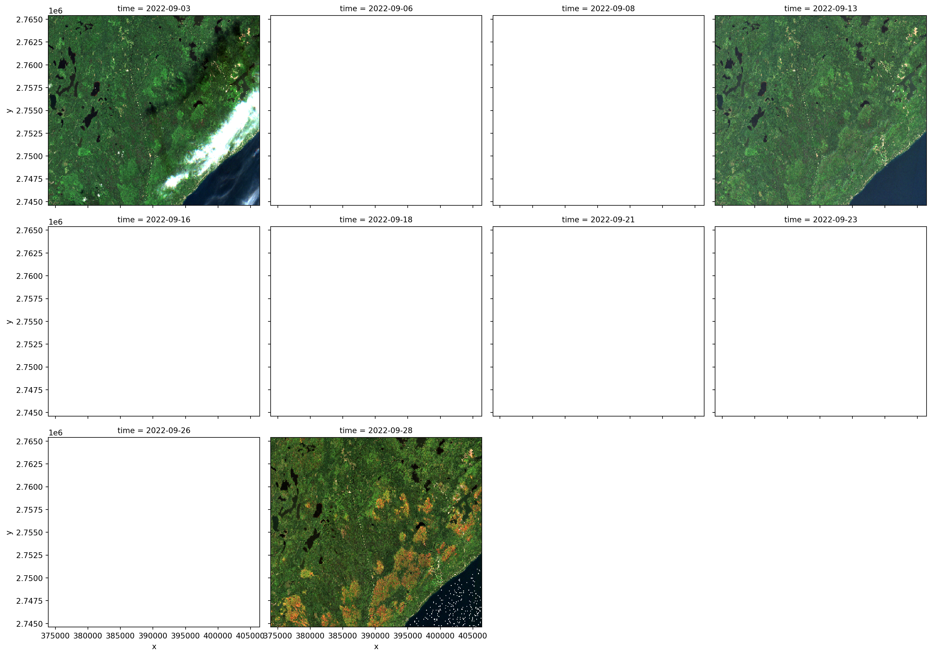
We can view the images easily with the plot method, giving us a glimpse into autumn on the North Shore of Lake Superior!

flat_stack.sel(band=["B04", "B03", "B02"]).plot.imshow(
    col="time",
    col_wrap=4,
    rgb="band",
    robust=True,
    size=4,
    vmin=0,
    vmax=1000,
    add_labels=False,
)

<xarray.plot.facetgrid.FacetGrid at 0x7f194cd13dd0>

/opt/hostedtoolcache/Python/3.11.4/x64/lib/python3.11/site-packages/matplotlib/cm.py:478: RuntimeWarning: invalid value encountered in cast
  xx = (xx * 255).astype(np.uint8)

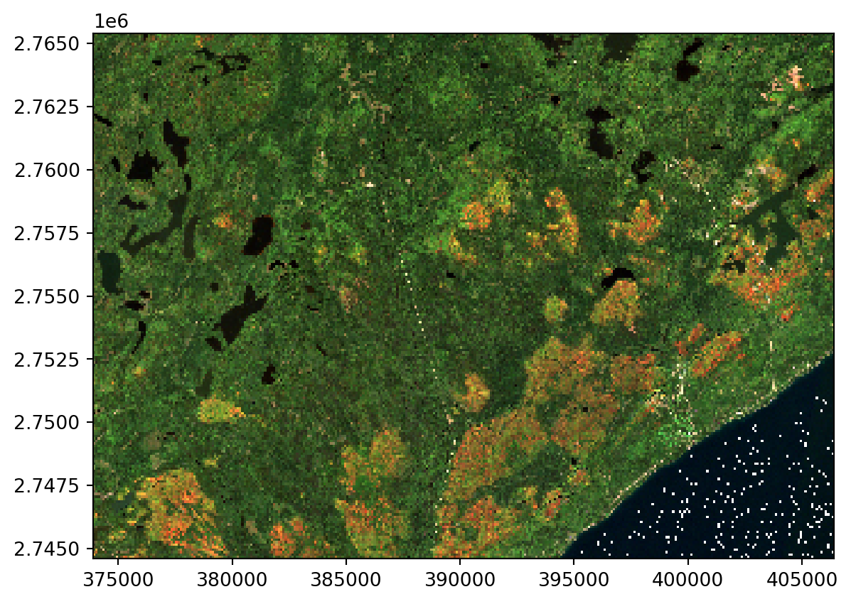
I remember it being cloudy last fall but damn we had a couple of nice days! Apparently September 28 was a really good one.

flat_stack.sel(band=["B04", "B03", "B02"], time="2022-09-28").plot.imshow(
    rgb="band",
    robust=True,
    size=5,
    vmin=0,
    vmax=1000,
    add_labels=False,
)

<matplotlib.image.AxesImage at 0x7f1910230290>

/opt/hostedtoolcache/Python/3.11.4/x64/lib/python3.11/site-packages/matplotlib/cm.py:478: RuntimeWarning: invalid value encountered in cast
  xx = (xx * 255).astype(np.uint8)

Whats next?

This is really just scratching the surface of what you can do with xarray, I will try to cover some more advanced topics in later posts.