HLS: Your new favorite remote sensing dataset

The Harmonized Landsat Sentinel 2 (HLS) dataset is an awesome public source for 30 meter spectral satellite imagery.

Sentinel 2 L2A

Landsat Collection 2 Level-2

 

Harmonized Landsat Sentinel 2

 

Produced by NASA, the HLS dataset combines the independently powerful Landsat 8/9 and Sentinel 2 satellite observation systems into one analysis-ready dataset.

Some of the best features include:

• More rich time series than either Sentinel 2 or Landsat individually

  • one observation every two to three days from HLS compared to one every five days for Sentinel 2 and one every eight days for Landsat 8/9

• It is BRDF corrected, which makes mosaics generated across orbits from different days nearly seamless

  • neither of the original data sources for Landsat or Sentinel data have this feature

• The data are accessible via NASA’s LPCLOUD STAC!

• Improved cloud masking for Sentinel 2!

  • The original Sentinel 2 cloud mask leaves something to be desired, but in the HLS collection you get a more robust mask that is consistent with the Landsat products

In this post, I am going to demonstrate some of the awesome capabilities of the HLS data and show why you should consider using it in place of either Landsat or Sentinel 2! Check out the HLS 2.0 User Guide for more details on the process for generating the HLS data.

Get organized

authentication with Earthdata and the .netrc file

To access the HLS data from NASA, you will need to have a (free) Earthdata Login profile. You can create an account here. Once your account is active, you will need to add your login credentials to a .netrc file in your home directory. You can do this with a single shell command in a Unix system:

echo "machine urs.earthdata.nasa.gov login <USERNAME> password <PASSWORD>" > ~/.netrc

When GDAL reads the raster data using curl it will find your credentials in this file.

environment variables

There are a handful of environment variables that must be set in order for GDAL to locate and read the raster files correctly. You can choose to include these in a startup script (e.g. ~/.bashrc) or set them within your Python script:

CPL_VSIL_CURL_USE_HEAD=FALSE
GDAL_DISABLE_READDIR_ON_OPEN=YES
GDAL_HTTP_COOKIEJAR=/tmp/cookies.txt
GDAL_HTTP_COOKIEFILE=/tmp/cookies.txt

imports

Here are the python packages that we need:

import datetime
import itertools
from collections import defaultdict

import pandas as pd
import pyproj
import pystac
import pystac_client
import stackstac
import xarray as xr
from rasterio.enums import Resampling
from shapely.geometry import box
from shapely.ops import transform

connect to the NASA STAC

The HLS data queried from the LPCLOUD STAC. We can use pystac_client to open a connection to the STAC:

CMR_STAC_URL = "https://cmr.earthdata.nasa.gov/stac/LPCLOUD"

catalog = pystac_client.Client.open(CMR_STAC_URL)

The HLS data are stored in two separate collections:

• Landsat: HLSL30.v2.0

• Sentinel: HLSS30.v2.0

HLS_COLLECTION_IDS = ["HLSL30.v2.0", "HLSS30.v2.0"]

There may be good reasons to keep them separate but this difference and one other design choice that we will discuss later make it more tedious to get up and running with the HLS data than it should!

area of interest

For this analysis we are going to focus on a section of the Kawishiwi River system on the edge of the Boundary Waters Canoe Area Wilderness in Northern Minnesota that I know as “the Little Triangle”.

# my CRS of choice for CONUS these days
CRS_STRING = "epsg:5070"
EPSG = pyproj.CRS.from_string(CRS_STRING).to_epsg()

# bounding box that surrounds the Little Triangle
AOI = box(326000, 2771000, 337000, 2778000)

# STAC items store bounding box info in epsg:4326
transformer_4326 = pyproj.Transformer.from_crs(
    crs_from=CRS_STRING,
    crs_to="epsg:4326",
    always_xy=True,
)

bbox_4326 = transform(transformer_4326.transform, AOI).bounds

Explore the data

check out this time series!

We can query the STAC catalog for the entire time series by searching the catalog without a datetime specification.

hls_history_search = catalog.search(
    collections=HLS_COLLECTION_IDS,
    bbox=bbox_4326,
)

all_items = []
for page in hls_history_search.pages():
    all_items.extend(page.items)

collection_history = {
    collection: defaultdict(list) for collection in HLS_COLLECTION_IDS
}

for item in all_items:
    year_month = pd.Timestamp(item.datetime.date()) + pd.offsets.MonthEnd()
    entry = collection_history[item.collection_id][year_month]
    if (date := item.datetime.date()) not in entry:
        entry.append(date)

Note

I am looping through the pages() because the NASA STAC connection can be flaky sometimes and will give you 502 errors when you loop through a long list of items(). I don’t know why the pages() method is more stable, but it seems to work better for large queries like this.

Code

# get count of images by year/month/sensor
collection_counts = pd.DataFrame(
    {
        collection: {
            year_month: len(dates) for year_month, dates in year_months.items()
        }
        for collection, year_months in collection_history.items()
    }
).fillna(0)

_ = collection_counts.plot.line(
    title="monthly count of days with observations by sensor"
)

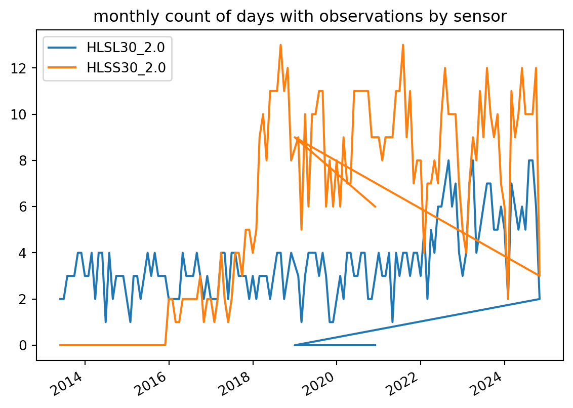
You can see that the Landsat time series stretches back to Landsat 8’s launch in 2013 and that the Sentinel 2 observations kick into gear in late 2020. The density of observations really ramped up in 2022 when Landsat 9 came online!

Note

NASA is currently working on adding the full Sentinel 2 archive (back to 2015) to the HLS dataset. That project is scheduled to be complete in the Fall of 2023 according to this EarthData forum post

band labels

One thing that makes it harder to get up and running with the HLS data is that the Sentinel and Landsat STAC items have different band IDs for the many of the spectral bands! This matters to us here because stackstac uses the STAC items’ asset labels to name the band dimension. Without any modifications, some of the bands would get scrambled when combining data from the two collections.

	Band name	OLI band number	MSI band number	HLS band code name L8	HLS band code name S2	Wavelength (micrometers)
0	Coastal Aerosol	1	1	B01	B01	0.43 – 0.45*
1	Blue	2	2	B02	B02	0.45 – 0.51*
2	Green	3	3	B03	B03	0.53 – 0.59*
3	Red	4	4	B04	B04	0.64 – 0.67*
4	Red-Edge 1	–	5	–	B05	0.69 – 0.71**
5	Red-Edge 2	–	6	–	B06	0.73 – 0.75**
6	Red-Edge 3	–	7	–	B07	0.77 – 0.79**
7	NIR Broad	–	8	–	B08	0.78 –0.88**
8	NIR Narrow	5	8A	B05	B8A	0.85 – 0.88*
9	SWIR 1	6	11	B06	B11	1.57 – 1.65*
10	SWIR 2	7	12	B07	B12	2.11 – 2.29*
11	Water vapor	–	9	–	B09	0.93 – 0.95**
12	Cirrus	9	10	B09	B10	1.36 – 1.38*
13	Thermal Infrared 1	10	–	B10	–	10.60 – 11.19*
14	Thermal Infrared 2	11	–	B11	–	11.50 – 12.51*

To avoid this headache, we can make define a crosswalk dictionary that will make it possible to modify the STAC item metadata so that we can safely load all of the data without scrambling the bands.

BAND_CROSSWALK = {
    "HLSL30.v2.0": {
        "B01": "coastal aerosol",
        "B02": "blue",
        "B03": "green",
        "B04": "red",
        "B05": "nir narrow",
        "B06": "swir 1",
        "B07": "swir 2",
        "B09": "cirrus",
        "B10": "thermal infrared 1",
        "B11": "thermal",
    },
    "HLSS30.v2.0": {
        "B01": "coastal aerosol",
        "B02": "blue",
        "B03": "green",
        "B04": "red",
        "B05": "red-edge 1",
        "B06": "red-edge 2",
        "B07": "red-edge 3",
        "B08": "nir broad",
        "B8A": "nir narrow",
        "B09": "water vapor",
        "B10": "cirrus",
        "B11": "swir 1",
        "B12": "swir 2",
    },
}

# these are the ones that we are going to use
BANDS = ["red", "green", "blue", "Fmask"]

Make a cloud-free mosaic

search the STAC

Now we are going to search the STAC again but this time with a datetime specification to limit our search to July 2022.

START_DATE = "2022-07-01"
END_DATE = "2022-07-31"

stac_items = catalog.search(
    collections=HLS_COLLECTION_IDS,
    bbox=bbox_4326,
    datetime=[START_DATE, END_DATE],
).item_collection()

modify the asset labels

We can use the crosswalk to rename the STAC item asset labels to pave the way for stackstac to load the data in the most convenient and straightforward way. There are ways to do this after you load the data using xarray.DataArray.assign_coords, but I find the STAC item metadata alteration approach more intuitive.

for item in stac_items:
    for original_band, new_band in BAND_CROSSWALK.get(item.collection_id).items():
        item.assets[new_band] = item.assets.pop(original_band)

load into a DataArray

Use stackstac.stack to load the STAC items into a neatly packaged xarray.DataArray:

hls_stack_raw = stackstac.stack(
    stac_items,
    assets=BANDS,
    bounds=AOI.bounds,
    epsg=EPSG,
    resolution=30,
    xy_coords="center",
)

/opt/hostedtoolcache/Python/3.11.4/x64/lib/python3.11/site-packages/stackstac/prepare.py:363: UserWarning: The argument 'infer_datetime_format' is deprecated and will be removed in a future version. A strict version of it is now the default, see https://pandas.pydata.org/pdeps/0004-consistent-to-datetime-parsing.html. You can safely remove this argument.
  times = pd.to_datetime(

cloud/shadow masking

The Fmask band contains all of the pixel quality information that we need to mask out invalid pixels from the images, but it takes a little bit of work. The quality information is stored in integer form but we can work with it using some binary tricks!

	Bit number	Mask name	Bit value	Mask description
0	6-7	aerosol level	11	High aerosol
1			10	Moderate aerosol
2			01	Low aerosol
3			00	Climatology aerosol
4	5	Water	1	Yes
5			0	No
6	4	Snow/ice	1	Yes
7			0	No
8	3	Cloud shadow	1	Yes
9			0	No
10	2	Adjacent to cloud/shadow	1	Yes
11			0	No
12	1	Cloud	1	Yes
13			0	No
14	0	Cirrus	Reserved, but not used

We can use the ‘bitwise OR’ operator | and the ‘zero fill left shift’ operator << to construct an integer representation of invalid pixels. For the cloud-free mosaic, we want to exclude any pixel that is marked (bit value = 1) as either a cloud (bit 1), adjacent to a cloud or shadow (bit 2), or a cloud shadow (bit 3).

hls_mask_bitfields = [1, 2, 3]  # cloud shadow, adjacent to cloud shadow, cloud
hls_bitmask = 0
for field in hls_mask_bitfields:
    hls_bitmask |= 1 << field

print(hls_bitmask)

14

If we cast the result to a binary string you can see how that works:

format(hls_bitmask, "08b")

'00001110'

When you translate the integer 14 into binary you get the ultimate invalid pixel!

Next, we use ‘bitwise AND’ to identify pixels that have an invalid value in any of the bits that we care about. Any integer value that has the invalid value (1) in any of the specified bits (1, 2, and 3) will return a non-zero value when compared to 14 with the & operator:

For example, a pixel where all bit values are zero will return zero because none of the bitwise 1 values are shared with our invalid mask value (14 aka 00001110):

int("00000000", 2) & 14

0

And a pixel that is marked as adjacent to a cloud or shadow (bit 2 = 1) will return 4 (2^2) because bit 2 has 1:

int("00000100", 2) & 14

4

Fortunately for us, we can apply the bitwise operators on integer arrays! We can classify all pixels as either good or bad like this:

fmask = hls_stack_raw.sel(band="Fmask").astype("uint16")
hls_bad = fmask & hls_bitmask

Then we can set all invalid pixels (hls_bad != 0) to NaN like this:

# mask pixels where any one of those bits are set
hls_masked = hls_stack_raw.where(hls_bad == 0)

get the cloud-free mosaic

After we have eliminated the invalid pixels it is very easy to generate a cloud-free mosaic for a specific time range (e.g. monthly). For example, we can take the median value from all non-cloud/non-cloud shadow pixels within a given month with just a few lines of code.

hls_cloud_free = hls_masked.resample(time="1M").median(skipna=True).compute()

We are only looking at a single month here, but you could pass many months worth of STAC items to stackstac.stack and get a rich time series of cloud-free imagery using the exact same method.

Plot the image and bask in the cloud-free beauty:

Code

_ = (
    hls_cloud_free.squeeze(dim="time")
    .sel(band=["red", "green", "blue"])
    .plot.imshow(
        rgb="band",
        robust=True,
        size=6,
        add_labels=False,
        xticks=[],
        yticks=[],
    )
)

 

 

Compare to Sentinel 2 L2A and Landsat Collection 2 Level-2

The Landsat Collection Level-2 and Sentinel 2 Level 2A datasets are available in Microsoft’s Planetary Computer STAC. They are available in other STACs, too (e.g. Element84’s Earth Search Catalog), but the Planetary Computer catalog is really nice and the data are well- documented and have examples attached to many of the available collections.

Code

import planetary_computer


planetary_computer_catalog = pystac_client.Client.open(
    "https://planetarycomputer.microsoft.com/api/stac/v1",
    modifier=planetary_computer.sign_inplace,
)

sentinel_stac_items = planetary_computer_catalog.search(
    collections=["sentinel-2-l2a"],
    bbox=bbox_4326,
    datetime=[START_DATE, END_DATE],
).get_all_items()

sentinel_band_crosswalk = {
    "B04": "red",
    "B03": "green",
    "B02": "blue",
}

for item in sentinel_stac_items:
    for original_band, new_band in sentinel_band_crosswalk.items():
        item.assets[new_band] = item.assets.pop(original_band)


sentinel_stack = stackstac.stack(
    items=sentinel_stac_items,
    assets=["red", "green", "blue", "SCL"],
    epsg=EPSG,
    resolution=30,
    bounds=AOI.bounds,
    xy_coords="center",
    resampling=Resampling.bilinear,
)

# valid SCL values: 4: vegetation, 5: bare soils, 6: water, 11: snow or ice
# https://docs.digitalearthafrica.org/en/latest/data_specs/Sentinel-2_Level-2A_specs.html
valid_scl = [4, 5, 6, 11]

sentinel_cloud_free = (
    sentinel_stack.where(sentinel_stack.sel(band="SCL").isin(valid_scl))
    .sel(band=["red", "green", "blue"])
    .resample(time="1M")
    .median(skipna=True)
    .compute()
)

landsat_stac_items = planetary_computer_catalog.search(
    collections=["landsat-c2-l2"],
    bbox=bbox_4326,
    datetime=[START_DATE, END_DATE],
    query={"platform": {"neq": "landsat-7"}},  # skip Landsat 7 because stripes
).get_all_items()


landsat_stack = stackstac.stack(
    items=landsat_stac_items,
    assets=["red", "green", "blue", "qa_pixel"],
    epsg=EPSG,
    resolution=30,
    bounds=AOI.bounds,
    xy_coords="center",
    band_coords=False,
)

# following https://stackstac.readthedocs.io/en/latest/examples/gif.html#Mask-cloudy-pixels-using-the-QA-band:
# Make a bitmask---when we bitwise-and it with the data, it leaves just the 4 bits we care about
mask_bitfields = [1, 2, 3, 4]  # dilated cloud, cirrus, cloud, cloud shadow
bitmask = 0
for field in mask_bitfields:
    bitmask |= 1 << field

landsat_qa = landsat_stack.sel(band="qa_pixel").astype("uint16")
landsat_bad = landsat_qa & bitmask  # just look at those 4 bits

landsat_good = landsat_stack.where(
    landsat_bad == 0
)  # mask pixels where any one of those bits are set

landsat_cloud_free = (
    landsat_good.sel(band=["red", "green", "blue"])
    .resample(time="1M")
    .median(skipna=True)
    .compute()
)

Both of the original datasets are atmospherially corrected and represent surface surface reflectance, but the processed images are definitely not free of cloud- or orbit artifacts! One of the greatest advantages of using the HLS dataset instead of the original sources is improved cloud masking. The HLS data undergo an entirely different process than the Landsat Collection Level-2 and Sentinel 2 Level 2A datasets, see below for an outline of the processing workflow.

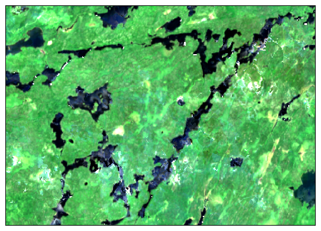
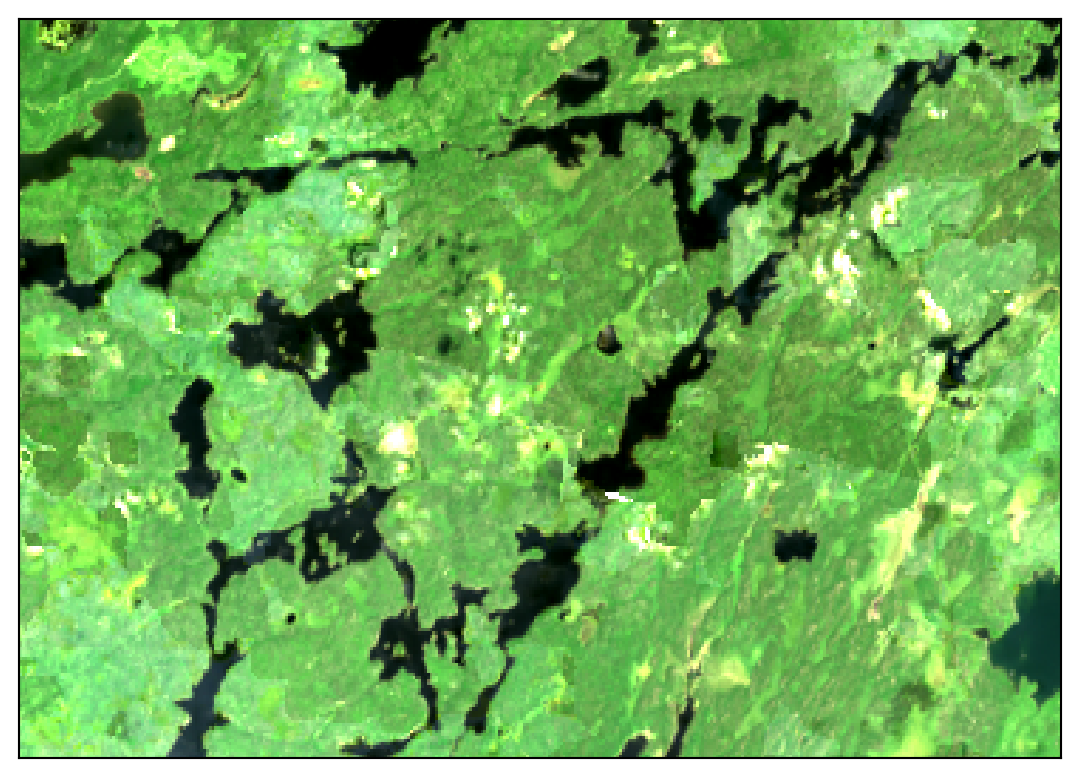
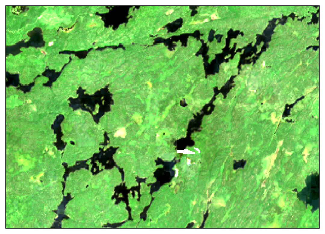
These images show 30 meter resolution, cloud-free mosaics for July 2022 from each source:

Figure 1: Sentinel 2

Figure 2: Landsat 8/9

 

Figure 3: Harmonized

 

In the Sentinel 2 image you can clearly see some cloud haze scattered around most of the image. The Landsat image shows patchy artifacts that are probably attributable to hazy clouds that were not masked from the original images. Meanwhile, the HLS mosaic comes out crystal clear!

Analyze the HLS Landsat and Sentinel collections separately

To illustrate the power of the full HLS dataset and the advantage of the high density of collections in a short time, lets load the imagery for each sensor separately and create a cloud-free mosaic for July 2022 for each one.

get an array for each sensor

items_by_collection = {
    collection: pystac.ItemCollection(
        [item for item in stac_items if item.collection_id == collection]
    )
    for collection in HLS_COLLECTION_IDS
}

stacks_by_collection = {}


# a function to flatten the time dimension
def flatten(x, dim="time"):
    assert isinstance(x, xr.DataArray)
    if len(x[dim].values) > len(set(x[dim].values)):
        x = x.groupby(dim).map(stackstac.mosaic)

    return x


for collection, collection_items in items_by_collection.items():
    raw_stack = stackstac.stack(
        collection_items,
        assets=BANDS,
        bounds=AOI.bounds,
        epsg=EPSG,
        resolution=30,
        xy_coords="center",
    )

    stacks_by_collection[collection] = flatten(raw_stack, dim="time")

/opt/hostedtoolcache/Python/3.11.4/x64/lib/python3.11/site-packages/stackstac/prepare.py:363: UserWarning: The argument 'infer_datetime_format' is deprecated and will be removed in a future version. A strict version of it is now the default, see https://pandas.pydata.org/pdeps/0004-consistent-to-datetime-parsing.html. You can safely remove this argument.
  times = pd.to_datetime(
/opt/hostedtoolcache/Python/3.11.4/x64/lib/python3.11/site-packages/stackstac/prepare.py:363: UserWarning: The argument 'infer_datetime_format' is deprecated and will be removed in a future version. A strict version of it is now the default, see https://pandas.pydata.org/pdeps/0004-consistent-to-datetime-parsing.html. You can safely remove this argument.
  times = pd.to_datetime(

We can combine them along a new dimension called sensor to make it easy to look at the images with respect to sensor and time.

sensor_stack = xr.concat(
    list(stacks_by_collection.values()),
    dim=pd.Index(["Landsat", "Sentinel"], name="sensor"),
)
sensor_stack

<xarray.DataArray 'stackstac-c6f93a695d3c1cd2194ae9ad1147db6e' (sensor: 2,
                                                                time: 26,
                                                                band: 4,
                                                                y: 234, x: 368)>
dask.array<concatenate, shape=(2, 26, 4, 234, 368), dtype=float64, chunksize=(1, 2, 1, 234, 368), chunktype=numpy.ndarray>
Coordinates:
  * band            (band) <U5 'red' 'green' 'blue' 'Fmask'
  * x               (x) float64 3.26e+05 3.26e+05 ... 3.37e+05 3.37e+05
  * y               (y) float64 2.778e+06 2.778e+06 ... 2.771e+06 2.771e+06
  * time            (time) datetime64[ns] 2022-07-03T17:20:28.306000 ... 2022...
    epsg            int64 5070
    id              (time) object 'HLS.S30.T15UXP.2022184T170901.v2.0' ... nan
    start_datetime  (time) object '2022-07-03T17:20:28.306Z' ... nan
    end_datetime    (time) object '2022-07-03T17:20:28.306Z' ... nan
    eo:cloud_cover  (time) float64 83.0 94.0 98.0 nan nan ... 77.0 57.0 29.0 nan
  * sensor          (sensor) object 'Landsat' 'Sentinel'
Attributes:
    spec:        RasterSpec(epsg=5070, bounds=(325980, 2770980, 337020, 27780...
    crs:         epsg:5070
    transform:   | 30.00, 0.00, 325980.00|\n| 0.00,-30.00, 2778000.00|\n| 0.0...
    resolution:  30

xarray.DataArray

'stackstac-c6f93a695d3c1cd2194ae9ad1147db6e'

• sensor: 2
• time: 26
• band: 4
• y: 234
• x: 368

• dask.array<chunksize=(1, 1, 1, 234, 368), meta=np.ndarray>

  Array Chunk Bytes 136.65 MiB 1.31 MiB Shape (2, 26, 4, 234, 368) (1, 2, 1, 234, 368) Dask graph 200 chunks in 62 graph layers Data type float64 numpy.ndarray

• Coordinates: (10)
  • band
    (band)
    <U5
    'red' 'green' 'blue' 'Fmask'

    array(['red', 'green', 'blue', 'Fmask'], dtype='<U5')

  • x
    (x)
    float64
    3.26e+05 3.26e+05 ... 3.37e+05

    array([325995., 326025., 326055., ..., 336945., 336975., 337005.])

  • y
    (y)
    float64
    2.778e+06 2.778e+06 ... 2.771e+06

    array([2777985., 2777955., 2777925., ..., 2771055., 2771025., 2770995.])

  • time
    (time)
    datetime64[ns]
    2022-07-03T17:20:28.306000 ... 2...

    array(['2022-07-03T17:20:28.306000000', '2022-07-03T17:20:32.409000000',
           '2022-07-05T17:10:27.219000000', '2022-07-07T16:58:04.238000000',
           '2022-07-08T16:51:29.257000000', '2022-07-08T17:20:20.107000000',
           '2022-07-08T17:20:24.204000000', '2022-07-10T17:10:31.859000000',
           '2022-07-13T17:20:27.894000000', '2022-07-13T17:20:31.994000000',
           '2022-07-15T16:57:38.356000000', '2022-07-15T17:10:23.464000000',
           '2022-07-15T17:10:26.655000000', '2022-07-16T16:51:52.688000000',
           '2022-07-18T17:20:20.078000000', '2022-07-18T17:20:24.176000000',
           '2022-07-20T17:10:33.633000000', '2022-07-23T16:58:09.629000000',
           '2022-07-24T16:52:00.788000000', '2022-07-25T17:10:24.008000000',
           '2022-07-25T17:10:27.200000000', '2022-07-28T17:20:20.229000000',
           '2022-07-28T17:20:24.328000000', '2022-07-30T17:10:28.776000000',
           '2022-07-30T17:10:31.960000000', '2022-07-31T16:58:17.249000000'],
          dtype='datetime64[ns]')

  • epsg
    ()
    int64
    5070

    array(5070)

  • id
    (time)
    object
    'HLS.S30.T15UXP.2022184T170901.v...

    array(['HLS.S30.T15UXP.2022184T170901.v2.0',
           'HLS.S30.T15UWP.2022184T170901.v2.0',
           'HLS.S30.T15UWP.2022186T165849.v2.0', nan, nan,
           'HLS.S30.T15UXP.2022189T170859.v2.0',
           'HLS.S30.T15UWP.2022189T170859.v2.0',
           'HLS.S30.T15UXP.2022191T165911.v2.0',
           'HLS.S30.T15UXP.2022194T170901.v2.0',
           'HLS.S30.T15UWP.2022194T170901.v2.0', nan,
           'HLS.S30.T15UXP.2022196T165849.v2.0',
           'HLS.S30.T15UWP.2022196T165849.v2.0', nan,
           'HLS.S30.T15UXP.2022199T170859.v2.0',
           'HLS.S30.T15UWP.2022199T170859.v2.0',
           'HLS.S30.T15UWP.2022201T165901.v2.0', nan, nan,
           'HLS.S30.T15UXP.2022206T165849.v2.0',
           'HLS.S30.T15UWP.2022206T165849.v2.0',
           'HLS.S30.T15UXP.2022209T170859.v2.0',
           'HLS.S30.T15UWP.2022209T170859.v2.0',
           'HLS.S30.T15UXP.2022211T165901.v2.0',
           'HLS.S30.T15UWP.2022211T165901.v2.0', nan], dtype=object)

  • start_datetime
    (time)
    object
    '2022-07-03T17:20:28.306Z' ... nan

    array(['2022-07-03T17:20:28.306Z', '2022-07-03T17:20:32.409Z',
           '2022-07-05T17:10:27.219Z', nan, nan, '2022-07-08T17:20:20.107Z',
           '2022-07-08T17:20:24.204Z', '2022-07-10T17:10:31.859Z',
           '2022-07-13T17:20:27.894Z', '2022-07-13T17:20:31.994Z', nan,
           '2022-07-15T17:10:23.464Z', '2022-07-15T17:10:26.655Z', nan,
           '2022-07-18T17:20:20.078Z', '2022-07-18T17:20:24.176Z',
           '2022-07-20T17:10:33.633Z', nan, nan, '2022-07-25T17:10:24.008Z',
           '2022-07-25T17:10:27.200Z', '2022-07-28T17:20:20.229Z',
           '2022-07-28T17:20:24.328Z', '2022-07-30T17:10:28.776Z',
           '2022-07-30T17:10:31.960Z', nan], dtype=object)

  • end_datetime
    (time)
    object
    '2022-07-03T17:20:28.306Z' ... nan

    array(['2022-07-03T17:20:28.306Z', '2022-07-03T17:20:32.409Z',
           '2022-07-05T17:10:27.219Z', nan, nan, '2022-07-08T17:20:20.107Z',
           '2022-07-08T17:20:24.204Z', '2022-07-10T17:10:31.859Z',
           '2022-07-13T17:20:27.894Z', '2022-07-13T17:20:31.994Z', nan,
           '2022-07-15T17:10:23.464Z', '2022-07-15T17:10:26.655Z', nan,
           '2022-07-18T17:20:20.078Z', '2022-07-18T17:20:24.176Z',
           '2022-07-20T17:10:33.633Z', nan, nan, '2022-07-25T17:10:24.008Z',
           '2022-07-25T17:10:27.200Z', '2022-07-28T17:20:20.229Z',
           '2022-07-28T17:20:24.328Z', '2022-07-30T17:10:28.776Z',
           '2022-07-30T17:10:31.960Z', nan], dtype=object)

  • eo:cloud_cover
    (time)
    float64
    83.0 94.0 98.0 ... 57.0 29.0 nan

    array([ 83.,  94.,  98.,  nan,  nan,  41.,  21., 100.,  33.,  13.,  nan,
            23.,   1.,  nan,  65.,  99.,  99.,  nan,  nan,  71.,  55.,  73.,
            77.,  57.,  29.,  nan])

  • sensor
    (sensor)
    object
    'Landsat' 'Sentinel'

    array(['Landsat', 'Sentinel'], dtype=object)

• Indexes: (5)
  • band
    PandasIndex

    PandasIndex(Index(['red', 'green', 'blue', 'Fmask'], dtype='object', name='band'))

  • x
    PandasIndex

    PandasIndex(Index([325995.0, 326025.0, 326055.0, 326085.0, 326115.0, 326145.0, 326175.0,
           326205.0, 326235.0, 326265.0,
           ...
           336735.0, 336765.0, 336795.0, 336825.0, 336855.0, 336885.0, 336915.0,
           336945.0, 336975.0, 337005.0],
          dtype='float64', name='x', length=368))

  • y
    PandasIndex

    PandasIndex(Index([2777985.0, 2777955.0, 2777925.0, 2777895.0, 2777865.0, 2777835.0,
           2777805.0, 2777775.0, 2777745.0, 2777715.0,
           ...
           2771265.0, 2771235.0, 2771205.0, 2771175.0, 2771145.0, 2771115.0,
           2771085.0, 2771055.0, 2771025.0, 2770995.0],
          dtype='float64', name='y', length=234))

  • time
    PandasIndex

    PandasIndex(DatetimeIndex(['2022-07-03 17:20:28.306000', '2022-07-03 17:20:32.409000',
                   '2022-07-05 17:10:27.219000', '2022-07-07 16:58:04.238000',
                   '2022-07-08 16:51:29.257000', '2022-07-08 17:20:20.107000',
                   '2022-07-08 17:20:24.204000', '2022-07-10 17:10:31.859000',
                   '2022-07-13 17:20:27.894000', '2022-07-13 17:20:31.994000',
                   '2022-07-15 16:57:38.356000', '2022-07-15 17:10:23.464000',
                   '2022-07-15 17:10:26.655000', '2022-07-16 16:51:52.688000',
                   '2022-07-18 17:20:20.078000', '2022-07-18 17:20:24.176000',
                   '2022-07-20 17:10:33.633000', '2022-07-23 16:58:09.629000',
                   '2022-07-24 16:52:00.788000', '2022-07-25 17:10:24.008000',
                   '2022-07-25 17:10:27.200000', '2022-07-28 17:20:20.229000',
                   '2022-07-28 17:20:24.328000', '2022-07-30 17:10:28.776000',
                   '2022-07-30 17:10:31.960000', '2022-07-31 16:58:17.249000'],
                  dtype='datetime64[ns]', name='time', freq=None))

  • sensor
    PandasIndex

    PandasIndex(Index(['Landsat', 'Sentinel'], dtype='object', name='sensor'))

• Attributes: (4)

  spec :

  RasterSpec(epsg=5070, bounds=(325980, 2770980, 337020, 2778000), resolutions_xy=(30, 30))

  crs :

  epsg:5070

  transform :

  | 30.00, 0.00, 325980.00| | 0.00,-30.00, 2778000.00| | 0.00, 0.00, 1.00|

  resolution :

  30

Since we are going to make several plots using this array, load the data into memory with a call to the .compute() method.

sensor_stack = sensor_stack.compute()

The HLS data are organized by 100 km MGRS tiles, and there can be redundant coverage by separate STAC items. We can clean this up by flattening the data out to have one observation per sensor per day.

# a function to prepare the arrays for better plotting
def flatten_by_day(x):
    return (
        x.assign_coords(time=x.time.astype("datetime64[D]"))
        .groupby("time")
        .map(stackstac.mosaic)
    )


flattened_by_day = xr.concat(
    [
        flatten_by_day(sensor_stack.sel(sensor=sensor))
        for sensor in ["Landsat", "Sentinel"]
    ],
    dim="sensor",
)

/tmp/ipykernel_6857/795691738.py:4: UserWarning: Converting non-nanosecond precision datetime values to nanosecond precision. This behavior can eventually be relaxed in xarray, as it is an artifact from pandas which is now beginning to support non-nanosecond precision values. This warning is caused by passing non-nanosecond np.datetime64 or np.timedelta64 values to the DataArray or Variable constructor; it can be silenced by converting the values to nanosecond precision ahead of time.
  x.assign_coords(time=x.time.astype("datetime64[D]"))
/tmp/ipykernel_6857/795691738.py:4: UserWarning: Converting non-nanosecond precision datetime values to nanosecond precision. This behavior can eventually be relaxed in xarray, as it is an artifact from pandas which is now beginning to support non-nanosecond precision values. This warning is caused by passing non-nanosecond np.datetime64 or np.timedelta64 values to the DataArray or Variable constructor; it can be silenced by converting the values to nanosecond precision ahead of time.
  x.assign_coords(time=x.time.astype("datetime64[D]"))

When we plot the images we only have one observation per day per sensor.

_ = flattened_by_day.sel(band=["red", "green", "blue"]).plot.imshow(
    col="sensor",
    row="time",
    rgb="band",
    robust=True,
    size=5,
    vmin=0,
    vmax=800,
    add_labels=False,
    xticks=[],
    yticks=[],
)

Check out the valid/invalid binary values for each sensor/date:

has_data = flattened_by_day.sel(band="red").isnull() == False
fmask = flattened_by_day.sel(band="Fmask").astype("uint16")
hls_bad = (fmask & hls_bitmask).where(has_data > 0)

_ = (
    (hls_bad > 0)
    .where(has_data > 0)
    .plot.imshow(
        col="sensor",
        row="time",
        size=4,
        add_labels=False,
        xticks=[],
        yticks=[],
    )
)

For illustration purposes, make a “combined” sensor array to add to sensor_stack

landsat = (
    sensor_stack.sel(sensor="Landsat")
    .assign_coords(sensor="combined")
    .expand_dims("sensor", 1)
)
sentinel = (
    sensor_stack.sel(sensor="Sentinel")
    .assign_coords(sensor="combined")
    .expand_dims("sensor", 1)
)
combined_stack = landsat.combine_first(sentinel)

full_stack = xr.concat([sensor_stack, combined_stack], dim="sensor")

Would we have at least one valid observation for every pixel?

# is there a non-na spectral observation?
has_data = full_stack.sel(band="red") > 0

# is the pixel invalid by our Fmask criteria?
fmask = full_stack.sel(band="Fmask").astype("uint16")
is_bad = fmask & hls_bitmask

# if not invalid and has non-na value it is valid
valid = (is_bad == 0).astype("float64").where(has_data > 0)

# are there any valid pixels in the time series?
has_valid = (valid > 0).any(dim="time")
_ = has_valid.plot.imshow(
    col="sensor",
    size=4,
    add_labels=False,
    vmin=0,
    vmax=1,
    xticks=[],
    yticks=[],
)

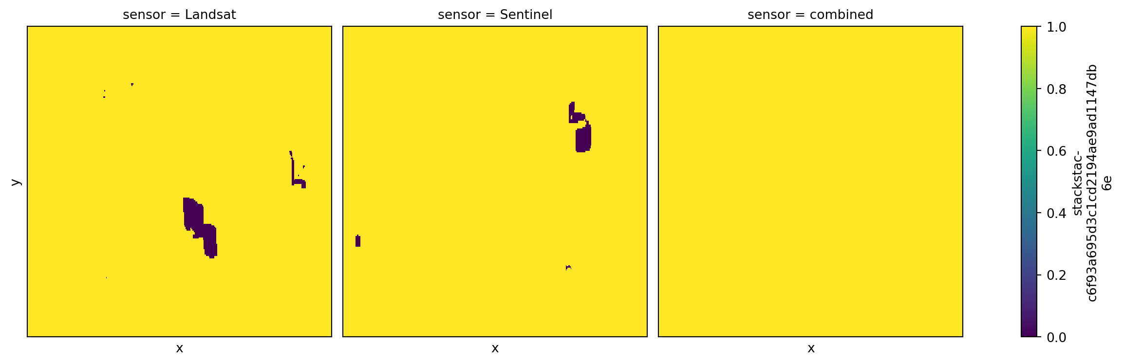
Not if we only use Landsat images, not if we use only Sentinel images, but we nearly have full coverage if we use the combined set!

(has_valid < 1).sum(dim=["x", "y"])

<xarray.DataArray 'stackstac-c6f93a695d3c1cd2194ae9ad1147db6e' (sensor: 3)>
array([1129,  603,    0])
Coordinates:
    epsg     int64 5070
  * sensor   (sensor) object 'Landsat' 'Sentinel' 'combined'

xarray.DataArray

'stackstac-c6f93a695d3c1cd2194ae9ad1147db6e'

• sensor: 3

• 1129 603 0

  array([1129,  603,    0])

• Coordinates: (2)
  • epsg
    ()
    int64
    5070

    array(5070)

  • sensor
    (sensor)
    object
    'Landsat' 'Sentinel' 'combined'

    array(['Landsat', 'Sentinel', 'combined'], dtype=object)

• Indexes: (1)
  • sensor
    PandasIndex

    PandasIndex(Index(['Landsat', 'Sentinel', 'combined'], dtype='object', name='sensor'))

• Attributes: (0)

By combining the sensors we reduce the number of pixels with no valid observations from hundreds down to only three!

Get cloud-free mosaic for each sensor and the combined set side-by-side.

sensor_cloud_free = full_stack.where(is_bad == 0).median(dim="time", skipna=True)

_ = sensor_cloud_free.sel(band=["red", "green", "blue"]).plot.imshow(
    col="sensor",
    rgb="band",
    robust=True,
    size=4,
    vmin=0,
    vmax=800,
    add_labels=False,
    xticks=[],
    yticks=[],
)

 

 

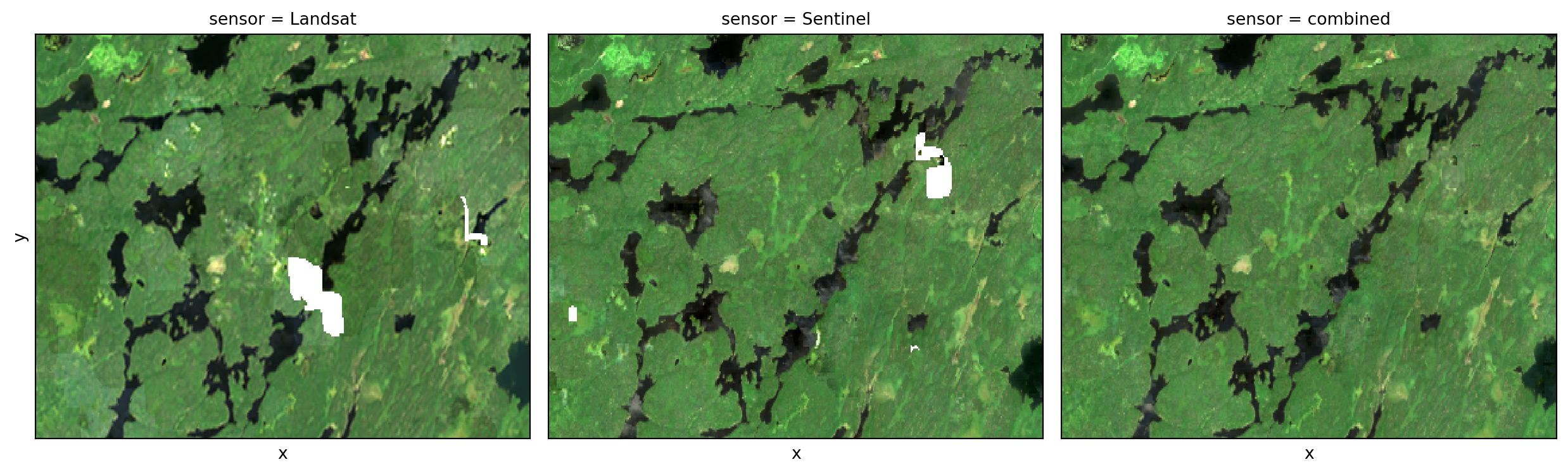
This demonstrates that combining the time series of observations from each of the sensor arrays gives you superior ingredients for cloud-free mosaic products than using either of the sensors independently.